A valuation model can look technically complete and still be wrong if the cost of equity is not defensible.

That is why the CAPM formula deserves attention before an analyst places it inside WACC, DCF, or an investment committee report.

The capital asset pricing model converts the return expectation of equity investors into a practical rate that can be used in valuation.

In a DCF model, that rate becomes the Ke input inside WACC when the model discounts FCFF.

In an equity-only valuation, it can also become the discount rate used to discount FCFE directly.

The problem is that many learners memorize the CAPM formula without reading what each component is actually doing.

They insert a risk-free rate, a beta, and an equity risk premium, then treat the output as if it were mechanically correct.

That is not how valuation works in practice.

A cost of equity formula is only as strong as the judgment behind its inputs.

This article explains the CAPM formula in three parts, then shows how NVIDIA can be used as a practical example for cost of equity estimation.

Section 1. CAPM Formula and the Cost of Equity Question

Every company raises capital from people who expect to be paid for risk.

Creditors expect contractual interest and principal repayment.

Shareholders accept a less certain claim, because they receive whatever remains after all other claims are satisfied.

The cost of equity is the return shareholders require for accepting that residual risk.

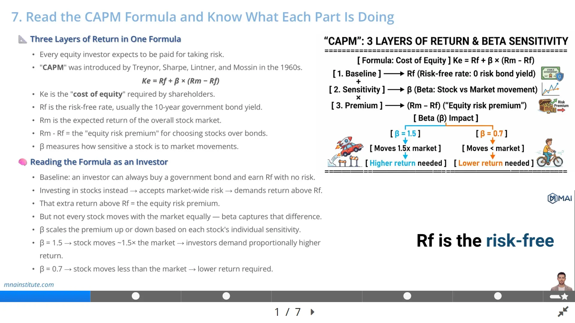
The CAPM formula estimates that required return by combining three layers of return.

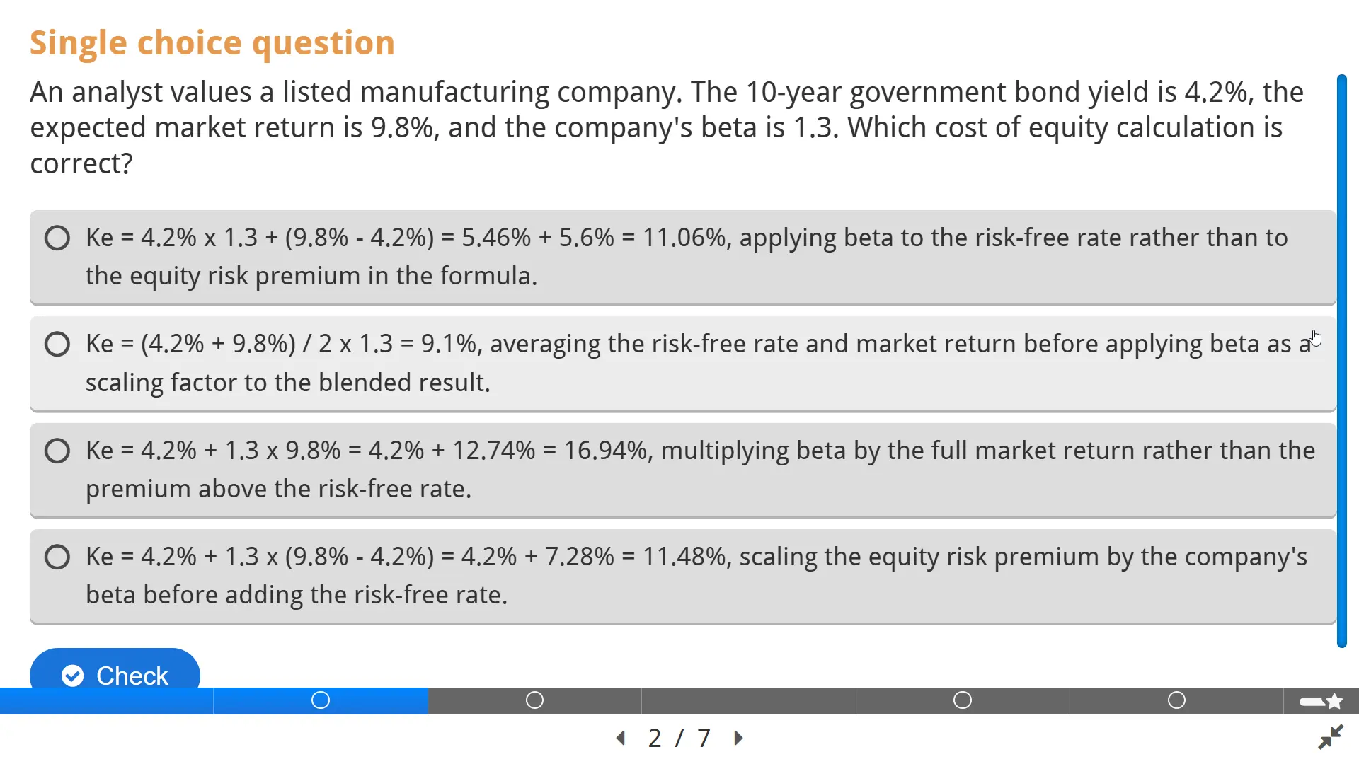
Ke = Rf + β × (Rm – Rf)

• Ke is the cost of equity.
• Rf is the risk-free rate.
• β is beta, which measures how sensitive the stock is to the broader market.
• Rm – Rf is the equity risk premium.

The formula says that shareholders first require a baseline return from a risk-free asset, then require extra compensation for equity market risk, adjusted by how much the specific stock moves with that market.

That is why the CAPM formula is not simply an academic expression.

It is a compact way to translate market risk into the return that equity investors demand.

The capital asset pricing model became widely used because it separates the cost of equity into observable or researchable inputs.

The analyst can source a government bond yield, estimate beta from share price history or data vendors, and use a published equity risk premium.

The difficulty is not writing the equation.

The difficulty is selecting inputs that match the company, country, currency, and forecast horizon being valued.

Section 2. Reading the CAPM Formula as an Investor

The easiest way to understand the CAPM formula is to read it from the viewpoint of an investor deciding whether to buy a stock.

The investor has a baseline alternative.

They can buy a government bond and earn the risk-free rate without accepting equity volatility.

That baseline is Rf.

If the investor buys the stock market instead, they accept market-wide risk.

They therefore require a premium above the bond yield.

That premium is Rm – Rf.

If the whole market requires a premium, the next question is whether the individual stock is riskier or more stable than the market.

Beta answers that question.

• A beta of 1.0 means the stock tends to move with the market.
• A beta of 1.5 means the stock has historically moved about 1.5 times as much as the market on average.
• A beta of 0.7 means the stock has historically moved less than the market.

The capital asset pricing model therefore scales the market premium up or down through beta.

This is why beta sits in the middle of the cost of equity formula.

It does not create risk by itself.

It measures how much market risk the specific stock brings into the investor portfolio.

For a large public company, this logic is usually sufficient because investors can diversify away many company-specific risks.

For smaller, private, illiquid, or highly concentrated businesses, the standard CAPM formula may need an additional risk adjustment.

Section 3. The Three Parts of the CAPM Formula

The CAPM formula has three practical inputs that must be selected with discipline.

Each input answers a different valuation question.

Input	Formula Role	Practical Question
Rf	Baseline return	What can investors earn before taking equity risk?
β	Risk scaling factor	How sensitive is this stock to the market?
Rm – Rf	Equity risk premium	What extra return does the market require over a safe bond?

Risk-Free Rate

The risk-free rate is the return an investor can earn without accepting default risk in the valuation currency.

For a US-listed company valued in US dollars, analysts commonly use a US Treasury yield.

The 10-year Treasury yield is often used because equity valuation is a long-horizon exercise and the exact holding period is usually uncertain.

For NVIDIA, the course example uses a 10-year US Treasury yield of 4.32 percent.

The key discipline is currency matching.

A dollar DCF should use a dollar risk-free rate.

A sterling DCF should use a sterling risk-free rate.

A Korean won DCF should use a won-denominated risk-free rate, adjusted carefully if sovereign default risk is embedded in the government bond yield.

Equity Risk Premium

The equity risk premium is the additional return investors expect from owning equities instead of safe government bonds.

It is written as Rm – Rf inside the CAPM formula.

This premium is not directly observable in the same way as a government bond yield.

Different estimation methods can produce different answers depending on the sample period, market index, arithmetic averaging, geometric averaging, and whether the estimate is historical or implied from current market prices.

That is why valuation practitioners typically use a published source rather than inventing an unsupported ERP inside the model.

Professor Aswath Damodaran publishes regularly updated implied equity risk premium data for the United States and country risk premium data for global markets.

The course example uses a US implied ERP of 4.90 percent from Damodaran.

Beta

Beta measures how sensitive a stock is to the broad equity market.

If beta is higher, the equity risk premium applied to that stock increases.

If beta is lower, the equity risk premium applied to that stock decreases.

A raw beta is usually estimated from historical stock returns against a market index.

Practitioners often adjust raw beta toward 1.0 because extreme historical beta estimates may partly reflect noise or temporary conditions.

The course example uses NVIDIA adjusted beta of 1.52 after applying an adjustment toward the market mean.

This beta means the model treats NVIDIA as more sensitive to market movements than the average listed company.

Section 4. How to Calculate Cost of Equity from CAPM

Once the inputs are selected, how to calculate cost of equity becomes straightforward.

The analyst multiplies beta by the equity risk premium, then adds the risk-free rate.

For NVIDIA in the course example, the inputs are as follows.

Input	Value	Interpretation
Rf	4.32%	10-year US Treasury yield used as the baseline dollar return
Adjusted β	1.52	NVIDIA market sensitivity after beta adjustment
ERP	4.90%	US implied equity risk premium used in the model
Ke	11.77%	Cost of equity produced by the CAPM formula

 

Ke = Rf + Adjusted β × ERP

Ke = 4.32% + 1.52 × 4.90%

Ke = 11.77%

The beta-adjusted equity premium is 7.45 percent.

That is the incremental return investors require for NVIDIA specific market sensitivity above the risk-free baseline.

Adding the 4.32 percent risk-free rate gives a final cost of equity of 11.77 percent.

In the WACC model, this number becomes Ke.

In a valuation memo, the analyst should not merely present the final number.

The analyst should show the input source, calculation logic, and reasonableness check.

That is the difference between a spreadsheet output and a defendable valuation assumption.

The same method can be applied to any listed company, provided the analyst chooses a consistent currency, a relevant risk-free rate, a reasonable ERP, and a defensible beta.

Section 5. When CAPM Needs an Adjustment

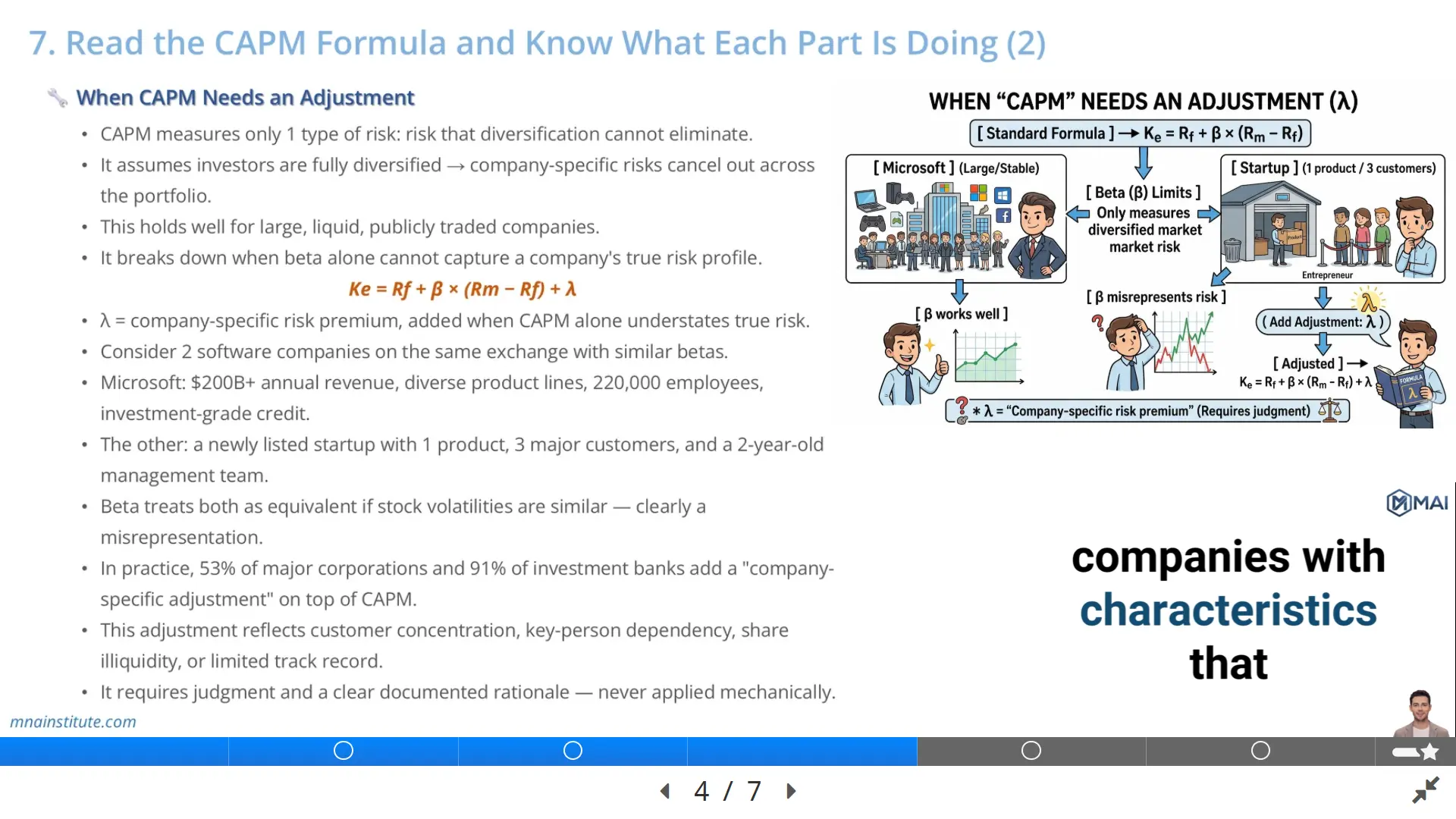
The standard CAPM formula assumes investors are diversified.

That means company-specific risk should not command extra return if investors can eliminate it through portfolio construction.

This assumption works reasonably well for large, liquid, publicly traded companies.

It becomes weaker when the company has risk characteristics that beta does not fully capture.

Examples include customer concentration, key-person dependency, limited trading liquidity, small scale, unstable operating history, or private company status.

In those cases, some analysts add a company-specific risk premium.

Ke = Rf + β × (Rm – Rf) + λ

The additional term λ represents the analyst judgment that CAPM alone understates the true required return.

This adjustment should not be used as a casual plug.

It should be supported by specific risk evidence.

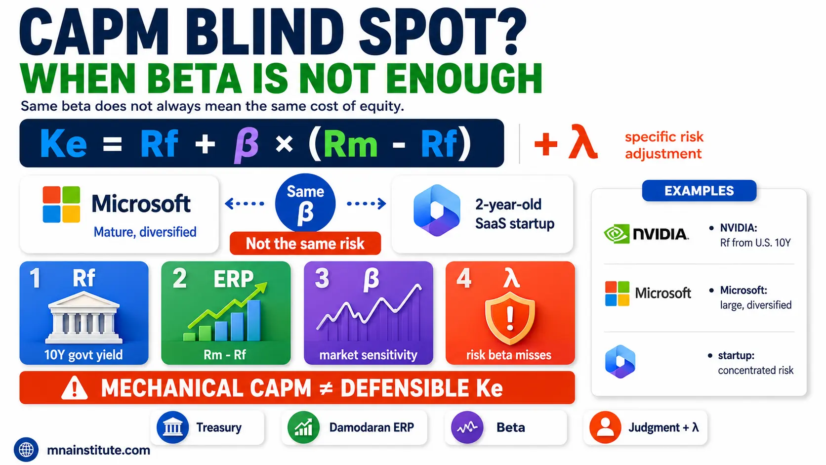
For example, consider two enterprise software companies listed on the same exchange with similar betas.

One is Microsoft, with more than 200 billion dollars in annual revenue, diversified products, global distribution, deep liquidity, and a long operating record.

The other is a newly listed software company with one flagship product, three customers, limited trading volume, and a management team with a short public company record.

If both companies show similar stock beta, a pure CAPM result could assign them nearly identical cost of equity.

That would fail to capture risk that does not appear cleanly in beta.

A company-specific premium can be appropriate when the analyst can explain the gap between market beta and actual business risk.

The adjustment belongs in a clearly documented valuation assumption, not as an unexplained number inserted to make the valuation look conservative.

Section 6. NVIDIA as a Practical CAPM Example

NVIDIA is a useful case because it combines exceptional growth, deep public market liquidity, large institutional ownership, and significant exposure to cyclical semiconductor demand.

The company is listed on Nasdaq and trades with high liquidity.

That makes a standard public-market CAPM approach more appropriate than a private-company cost of equity method.

In the course model, NVIDIA cost of equity is built from three sourced inputs.

• Risk-free rate: 4.32 percent from the 10-year US Treasury yield.
• Equity risk premium: 4.90 percent from Damodaran implied US ERP.
• Adjusted beta: 1.52 based on NVIDIA market sensitivity, adjusted toward 1.0.

The resulting Ke is 11.77 percent.

The number is high enough to reflect NVIDIA higher market sensitivity and semiconductor cyclicality.

It is not so high that it treats NVIDIA like an early-stage venture or illiquid private company.

That distinction matters.

NVIDIA may face business risks such as AI infrastructure demand cycles, customer concentration, export controls, supply chain constraints, and competitive pressure.

But the cost of equity model should not automatically add a company-specific premium for every risk mentioned in a 10-K.

For a large-cap public company, many risks are already reflected in market beta, analyst expectations, and the equity risk premium.

Adding λ on top of CAPM for NVIDIA would require a specific reason showing that beta and ERP materially understate the risk to diversified public equity holders.

In the course example, no additional premium is applied.

That is a reasonable approach for a large, liquid, widely followed public company.

Had the same business been a private semiconductor startup with no public trading record, concentrated customers, and limited financing history, the conclusion would be different.

The analyst would need to consider illiquidity, size, key-person risk, customer concentration, and lack of diversification.

Section 7. Verifying Whether the CAPM Result Is Reasonable

A calculated cost of equity should be checked before it enters a DCF model.

The first check is sensitivity.

If beta changes from 1.40 to 2.00, the cost of equity can move materially.

Using the same Rf and ERP, a beta of 1.40 produces a lower Ke than a beta of 2.00.

That sensitivity tells the analyst whether the valuation is highly dependent on the selected beta.

The second check is market comparison.

Equity research notes sometimes disclose WACC or cost of equity assumptions.

If the analyst cost of equity is far below or above the range used by market practitioners, the input selection should be reviewed.

The third check is business intuition.

A cost of equity below 8 percent for a high-growth semiconductor company would usually require a strong explanation.

A cost of equity above 18 percent for a large, profitable, liquid public company would also require a strong explanation.

The NVIDIA example of 11.77 percent sits within a plausible range for a listed company with high growth, significant market sensitivity, and capital-intensive industry exposure.

The final check is formula integrity.

The model should link Rf, beta, and ERP from clear input cells rather than hard-coding Ke directly.

That allows the analyst to update the risk-free rate, ERP, beta, and sensitivity table without breaking the model.

This is also where AI can assist without replacing judgment.

AI can help source the latest Treasury yield, locate Damodaran ERP data, explain beta adjustments, and compare industry assumptions.

The analyst must still verify every figure against the original source and decide whether the input is appropriate for the valuation case.

Section 8. Common CAPM Mistakes That Distort Valuation

Several CAPM mistakes repeat across beginner models and even some professional workpapers.

The first mistake is mixing currencies.

If the forecast is in US dollars, the risk-free rate and equity risk premium must also be dollar-based inputs.

Using a local government bond yield in one currency and cash flows in another currency creates a discount rate that does not match the valuation model.

The second mistake is confusing historical return with required return.

A stock may have performed exceptionally well in the past, but CAPM is not asking what the investor earned yesterday.

It asks what return equity holders require today for bearing forward-looking risk.

The third mistake is treating beta as a perfect measure of business risk.

Beta is a market sensitivity measure, not a complete operating risk map.

A company may have high customer concentration, heavy regulatory exposure, or technology disruption risk that beta does not express cleanly.

The fourth mistake is applying a company-specific risk premium without discipline.

A premium may be justified for private companies, thinly traded shares, early-stage businesses, or unusually concentrated operations.

It is much harder to justify for large liquid public companies unless the analyst can clearly explain why market beta and ERP fail to capture the risk.

The fifth mistake is failing to reconcile CAPM with the rest of the valuation.

A model that uses a high-growth revenue case, a low WACC, and a generous terminal growth rate can produce a valuation that looks precise but is internally aggressive.

CAPM should therefore be checked against the company story, peer risk, sensitivity analysis, and the final investment recommendation.

Section 9. How CAPM Connects to DCF and WACC

The CAPM formula usually enters the valuation workflow through WACC.

In an FCFF-based DCF model, the analyst discounts free cash flow to the firm at WACC to estimate enterprise value.

WACC includes the cost of equity and the after-tax cost of debt, weighted by market value capital structure.

That means a weak cost of equity estimate contaminates the entire DCF result.

If Ke is too low, WACC becomes too low, the present value of cash flows becomes too high, and the implied share price is overstated.

If Ke is too high, the valuation may understate the business even when the operating forecast is sound.

This is why cost of equity deserves the same scrutiny as revenue growth, EBIT margin, terminal value, and working capital assumptions.

In an FCFE valuation, the connection is even more direct.

Future free cash flow to equity is discounted at Ke rather than WACC.

In that case, the CAPM output is the discount rate that turns shareholder cash flows into equity value directly.

Either way, CAPM is not a detached finance theory topic.

It is a core valuation input that affects investment conclusion, bid range, and capital allocation decision.

Related Courses

The cost of equity formula is one component of a wider valuation workflow.

• Students who need the full path from filing review to DCF, CCA, WACC, sensitivity analysis, and report writing can use the Financial Modeling and Valuation Course with AI and Excel as the main curriculum.
• The Financial Statement Analysis Course with AI for Equity Research supports the first stage of valuation by teaching how to read 10-K filings, interpret financial statements, identify red flags, and convert accounting data into analyst judgment.
• The 3-Statement Financial Modeling Course with AI focuses on translating business research into forecast assumptions, linked statements, EPS, EBITDA, FCF, and model verification.
• For M&A professionals, the Mergers and Acquisitions Online Course, M&A Due Diligence Course, and Post Merger Integration Course connect valuation work to deal screening, diligence, transaction judgment, and post-closing execution.

Sources

• S. Department of the Treasury – Interest Rate Statistics
• Aswath Damodaran – Current Data and Equity Risk Premiums
• Bruner, Eades, Harris, and Higgins – Best Practices in Estimating the Cost of Capital
• NVIDIA Investor Relations – Financial Information