A DCF model does not end when the explicit forecast period ends.

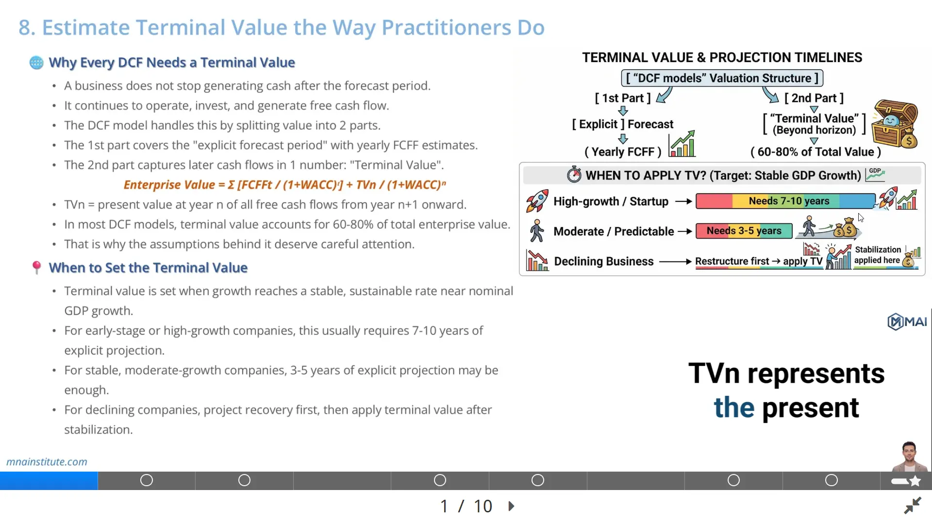
The company continues to operate, reinvest, and generate free cash flow after the final forecast year.

That continuing value has to be captured somewhere, and that is exactly what terminal value does.

The terminal value formula is the mechanism that converts all cash flows after the explicit projection period into a single value at the end of the forecast horizon.

This is where valuation judgment becomes much more visible than spreadsheet mechanics.

A model can have clean historical data, well-formatted schedules, and correct FCFF calculations, but still produce a weak valuation if the terminal value assumption is unrealistic.

That is why practitioners do not treat terminal value as the final line of the DCF.

They treat it as the part of the model where the business must prove that it has reached a stable state.

In a high-growth company, terminal value should not be applied before growth, margins, reinvestment, and returns on capital are reasonably mature.

In a mature company, the explicit forecast period may be shorter because the business is already close to long-run equilibrium.

In a declining company, the model may need a recovery or restructuring period before any perpetuity assumption can be defended.

This article explains the terminal value formula across three methods, the terminal growth rate discipline behind the Gordon Growth Model, and how the exit multiple method works in practical DCF modelling.

Why Every DCF Needs a Terminal Value

A DCF model values a business by discounting future free cash flows back to today.

The practical problem is that no analyst can forecast every year of a company forever.

The model solves this by separating value into two parts, and the terminal value formula connects the second part to the first.

The first part is the explicit forecast period, where FCFF is projected year by year.

The second part is terminal value, which captures the value of all cash flows beyond that forecast horizon.

In simplified form, Enterprise Value equals the present value of explicit FCFF plus the present value of terminal value.

Enterprise Value = Present value of explicit FCFF + Present value of terminal value.

The terminal value formula therefore sits inside the DCF model, not outside it.

It is not an optional add-on.

It is the valuation answer to a basic economic reality: the business does not stop after year five, year seven, or year ten.

For a going-concern company, the business should keep earning, investing, and producing cash flow after the explicit period.

If the DCF ignored that period, it would undervalue almost every continuing business.

The sensitivity of terminal value also explains why small changes in terminal growth rate can move the final valuation materially.

When terminal value represents a large share of enterprise value, the quality of the assumption matters as much as the accuracy of near-term forecasts.

A weak model hides that sensitivity.

A professional model exposes it, tests it, and explains it.

The terminal value formula is not just mathematics, and the terminal value formula should always be tested against the business model.

It is a statement about the long-term economics of the company being valued.

When to Set the Terminal Value

The most practical question is not which terminal value formula to use first, because the terminal value formula only becomes defensible after the business has stabilized.

The first question is when the terminal value should begin.

Terminal value should be estimated only after the company has reached a state that can support a stable long-term assumption.

That state is usually defined by four conditions.

1. Revenue growth has moved toward a sustainable long-run rate.
2. Margins have reached a level that can be defended beyond the explicit forecast period.
3. Reinvestment needs are consistent with the terminal growth rate.
4. Returns on capital are realistic in a competitive market.

This is why a mechanical five-year forecast can be dangerous.

A mature utility or consumer staples company may already be close to stability, so a shorter explicit forecast period can be acceptable.

A high-growth semiconductor or software company may require a much longer explicit period because growth, reinvestment, and competitive pressure have not yet normalized.

A venture-stage company may need an even longer path because free cash flow may be negative for several years before the business becomes self-funding.

A declining company requires a different logic again.

The model may need to show revenue pressure, cost restructuring, asset rationalization, and eventual stabilization before the terminal value assumption becomes credible.

The key is convergence.

The terminal value formula becomes more defensible when the final forecast year already resembles a sustainable business rather than a transitional one.

For example, assume a company grows FCFF at 25% for the next five years, but the analyst applies a 3% perpetuity growth rate immediately after year five.

That may look conservative because 3% is low.

But it can still be wrong if the business has not yet moved from exceptional growth to stable economics.

The model would be forcing a high-growth company into maturity too soon.

The result could understate value if the explicit period is too short, or overstate value if the terminal margin and reinvestment assumptions are too optimistic.

A reasonable terminal value process asks whether the business has actually reached a point where the chosen terminal growth rate makes sense.

This is the judgment behind the forecast horizon.

Business type	Typical terminal value timing logic	What the analyst must prove
Early-stage company	Longer explicit projection, often well beyond five years	The company can move from losses to positive sustainable FCFF
High-growth company	Explicit period extends until growth and reinvestment moderate	Growth converges toward a sustainable long-run rate
Mature company	Shorter explicit period may be enough	Margins, reinvestment, and returns are already stable
Declining company	Terminal value only after recovery or stabilization	The business has a defendable continuing base

Liquidation Value and Exit Multiple Method

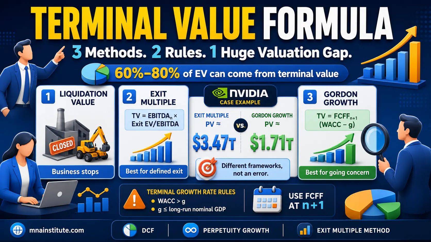
There are three broad ways to estimate terminal value.

The first is liquidation value.

The second is the exit multiple method.

The third is the Gordon Growth Model, also called the perpetuity growth model.

Each method answers a different economic question.

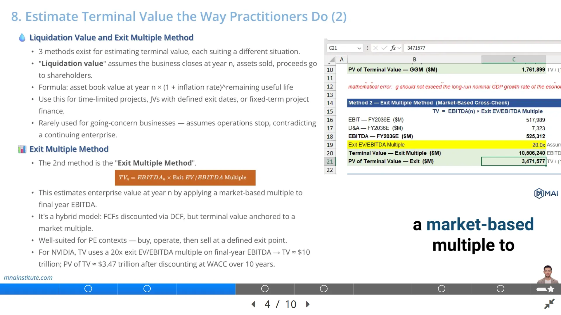
Liquidation value asks what the business would be worth if operations stopped and assets were sold.

The exit multiple method asks what a buyer might pay for the business at the end of the forecast period using a market multiple.

The Gordon Growth Model asks what the continuing stream of FCFF is worth if it grows at a stable rate forever.

Liquidation value

Liquidation value is rarely the right method for a normal going-concern company.

It assumes the business closes at the terminal date, sells its assets, repays liabilities, and distributes any remaining proceeds.

That assumption contradicts the central premise of most DCF models, which is that the business continues operating.

However, liquidation value can make sense in specific situations.

• A project finance asset with a fixed concession period.
• A joint venture with a defined exit date.
• A mine, field, or infrastructure asset with a finite economic life.
• A wind-down case where management has no credible continuing plan.

In those situations, the terminal value formula is not really a going-concern formula.

It is an asset realization estimate.

The analyst focuses on recoverable asset value, disposal costs, remaining liabilities, and timing of proceeds.

For most operating companies, the liquidation method is used more as a downside reference than as the primary valuation approach.

Exit Multiple Method

The exit multiple method is widely used because it is simple, market-based, and easy to explain to deal teams.

The terminal value formula under this method is straightforward, but the terminal value formula still depends on a defensible multiple.

Terminal Value = Final Year EBITDA × Exit EV to EBITDA Multiple.

The analyst estimates the company’s EBITDA in the final forecast year and applies a valuation multiple based on comparable companies, precedent transactions, or an expected exit environment.

This method is common in private equity because the investment thesis often involves buying the company, improving it, and selling it after a defined holding period.

In that context, the exit multiple method matches how the sponsor thinks about exit value.

The method is also used in investment banking because it can be tied to observable market multiples.

The advantage is practicality.

The disadvantage is that it can import market pricing into an intrinsic valuation model without fully explaining the long-term cash flow economics.

That is why the exit multiple method is best understood as a market cross-check rather than a pure intrinsic method.

A high exit multiple may be justifiable if the final-year business has superior growth, margins, returns on capital, and competitive position relative to peers.

A low exit multiple may be appropriate if the business is cyclical, structurally pressured, or dependent on unsustainable margins.

The exit multiple method should not be selected simply because it produces a desired valuation.

A defensible exit multiple must be connected to business quality, peer comparability, transaction conditions, and the final-year financial profile.

How to use the exit multiple method without making it arbitrary

The cleanest approach is to build a bridge between operating assumptions and the selected multiple.

If the final forecast year assumes 25% EBITDA growth, premium margins, and low reinvestment, but the exit multiple is based on mature peers growing at 5%, the analysis is inconsistent.

If the business is assumed to mature by the terminal year, the peer set should also represent mature operating economics.

For a private equity case, the exit multiple should reflect the likely buyer universe at exit, not just today’s public trading multiple.

For a strategic M&A case, it may be reasonable to test exit multiple sensitivity around current sector multiples and precedent transaction ranges.

The exit multiple method is useful because it forces the analyst to ask what the company could realistically be sold for at the end of the explicit forecast period.

It is dangerous when it becomes a plug that hides weak terminal economics.

The Gordon Growth Model

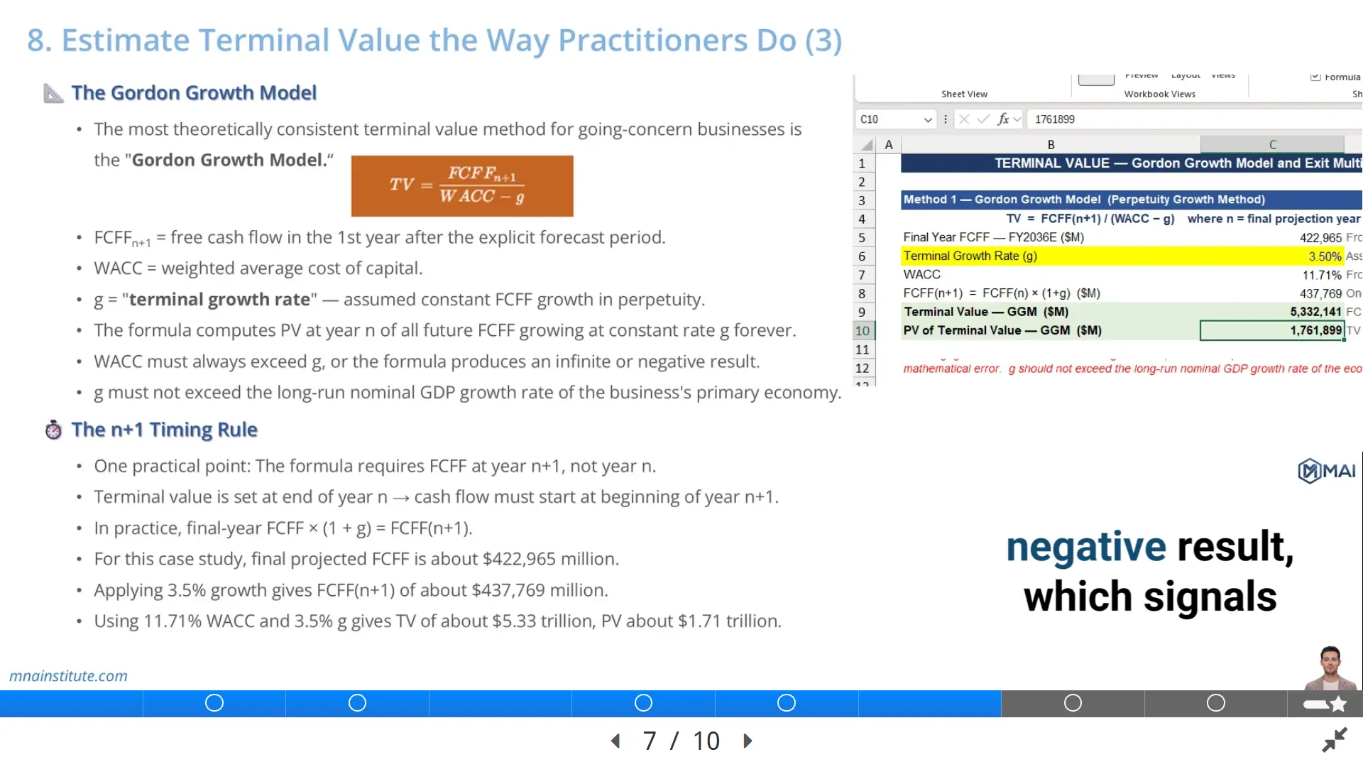
The Gordon Growth Model is the most theoretically consistent terminal value formula for a going-concern business, because the terminal value formula is tied directly to FCFF, WACC, and growth.

It is also called the perpetuity growth model.

The formula is simple.

Terminal Value = FCFF in year n plus 1 divided by WACC minus terminal growth rate.

Written more compactly,

TV = FCFFn+1 / WACC – g.

FCFFn+1 means the free cash flow expected in the first year after the explicit forecast period.

WACC is the discount rate applied to free cash flow to the firm.

g is the terminal growth rate.

The model assumes that FCFF grows at a constant rate forever after the explicit forecast period.

That assumption can be reasonable only if the company has reached stable economics by the terminal year.

The terminal growth rate should reflect long-run sustainable growth, not the company’s recent momentum.

For a company operating mainly in one economy, a common reference point is long-run nominal GDP growth in that economy.

The terminal growth rate should not exceed the long-run growth capacity of the economy in which the business primarily operates.

No individual company can grow faster than the economy forever without eventually becoming larger than the economy itself.

The other rule is mathematical.

WACC must be greater than terminal growth rate.

If terminal growth rate equals or exceeds WACC, the denominator becomes zero or negative, and the terminal value formula stops producing an economically meaningful answer.

This is not a spreadsheet error.

It is the model telling the analyst that the assumption is not defensible.

Terminal growth rate is a reinvestment assumption, not just a growth input

A common beginner mistake is to think of terminal growth rate as a standalone percentage.

In reality, growth requires reinvestment.

A company cannot grow FCFF forever without reinvesting in working capital, capital expenditure, acquisitions, R&D, or other operating assets.

If the terminal value formula assumes perpetual growth, the final-year model should also contain a reinvestment profile consistent with that growth.

A company that claims high perpetual growth with almost no reinvestment is implicitly assuming extraordinary returns on capital forever.

That may be possible for a short period, but it is difficult to defend permanently in a competitive market.

A professional valuation therefore checks three items together: terminal growth rate, reinvestment need, and return on capital.

If those three do not fit, the terminal value conclusion is weak even if the formula is correct.

The n+1 Timing Rule

The n+1 timing rule is one of the simplest details in terminal value modelling, but it is often missed.

The Gordon Growth Model uses the cash flow in the year after the explicit forecast period, so the terminal value formula must start with FCFFn+1.

If the explicit forecast ends in year n, the terminal value is measured at the end of year n.

The first cash flow included in the perpetuity is therefore year n plus 1.

That is why the formula uses FCFFn+1, not FCFFn.

In practice, the analyst takes the final projected FCFF and grows it by one year at the terminal growth rate.

FCFFn+1 = FCFFn × (1 + g).

Then the analyst divides FCFFn+1 by WACC minus g.

This detail matters because using FCFFn instead of FCFFn+1 understates terminal value by one year of growth.

The error may look small, but in a valuation where terminal value drives a large share of enterprise value, even small timing mistakes can move the implied share price.

The n+1 rule also helps analysts think correctly about what terminal value represents.

Terminal value is not the final-year cash flow.

It is the value at the end of the final year of all cash flows that begin after that year.

Example

Consider a simplified NVIDIA-style case based on the course example.

Assume the final projected FCFF in year 10 is $422,965 million.

Assume WACC is 11.71%.

Assume the terminal growth rate is 3.5%.

The first step is to apply the n+1 timing rule.

FCFFn+1 = $422,965 million × 1.035 = approximately $437,769 million.

The second step is to apply the Gordon Growth Model terminal value formula, which is the terminal value formula used for a stable going-concern case.

Terminal Value = $437,769 million / 11.71% – 3.5%.

The denominator is 8.21%.

That produces a terminal value of approximately $5.33 trillion at the end of year 10.

The third step is to discount that terminal value back to today using WACC over the 10-year forecast period.

In the course example, that produces a present value of terminal value of approximately $1.71 trillion.

Now compare that with the exit multiple method.

If the model applies a 20x exit EV to EBITDA multiple to the final projection year EBITDA, the terminal value is approximately $10 trillion.

Discounted at WACC over 10 years, the present value of terminal value is approximately $3.47 trillion.

The gap between the two methods is not a minor technical difference.

It tells the analyst that the valuation conclusion depends heavily on the terminal value method and assumption set.

That is exactly why a serious DCF model should show both methods and explain why one is more appropriate for the investment question.

Method	Core formula	Best use case	Main risk
Liquidation value	Asset value less liabilities and costs	Finite-life assets or wind-down cases	Not suitable for most going-concern businesses
Exit multiple method	Final-year EBITDA multiplied by exit EV to EBITDA multiple	Private equity exits and market-based cross-checks	Can become a market multiple plug
Gordon Growth Model	FCFFn+1 divided by WACC minus g	Stable going-concern businesses	Highly sensitive to terminal growth rate and WACC

 

How Practitioners Test the Terminal Value Formula

Practitioners rarely rely on a single terminal value output without testing it.

They usually review the implied economics behind the result.

A useful checklist includes the following questions.

• Does the final forecast year look like a stable business rather than a transition year?
• Is the terminal growth rate below a defensible long-run economic growth benchmark?
• Is WACC greater than terminal growth rate by a reasonable spread?
• Are reinvestment assumptions consistent with perpetual growth?
• Does the exit multiple align with the final-year growth, margins, and risk profile?
• Does the implied share price remain reasonable under sensitivity analysis?

The purpose of this checklist is not to make the model conservative by default.

The purpose is to make the terminal value formula economically consistent.

A company with exceptional competitive advantages may deserve a higher terminal value than an average company.

But the analyst must show why that advantage persists, how reinvestment supports future growth, and why returns on capital remain above the cost of capital.

The best terminal value analysis is not the one that produces the highest valuation.

It is the one that a valuation committee, investment committee, or transaction team can defend under questioning.

Related Courses

This article connects directly with the valuation workflow taught in the courses below.

• Financial Modeling and Valuation Course with AI and Excel: the full learning path from financial analysis to WACC, DCF, CCA, and valuation report.
• Financial Statement Analysis Course with AI for Equity Research: the foundation for reading filings, testing financial quality, and identifying valuation inputs.
• 3-Statement Financial Modeling Course with AI: the Excel modelling workflow that turns business drivers into FCFF, EBITDA, EPS, and scenarios.
• Mergers and Acquisitions Online Course: the broader transaction framework where valuation supports deal screening, due diligence, negotiation, and integration.
• M&A Due Diligence Course: the practical diligence process that tests whether assumptions behind the valuation can be trusted.
• Post Merger Integration Course: the value-up logic that connects deal rationale, synergy capture, and post-close execution.

Sources

• Aswath Damodaran, Closure in Valuation: Estimating Terminal Value
• Aswath Damodaran, The Stable Growth Rate
• CFA Institute, Equity Valuation learning outcomes, including terminal value and multiples in multistage DCF
• McKinsey, How to value cyclical companies