A completed DCF model can look precise because it produces one implied share price.

That precision can be misleading if the model does not show how the result changes when key assumptions move.

DCF sensitivity analysis exists to turn valuation uncertainty into a structured range of outcomes.

It shows how the implied share price reacts when WACC, terminal growth rate, revenue growth, EBIT margin, or exit multiple changes within a plausible range.

This matters because a valuation conclusion is rarely judged by whether one base case number is elegant.

It is judged by whether the analyst can explain the assumptions behind the upper and lower boundaries of the valuation range.

A serious model should therefore move from a single point estimate to a defensible set of cases that can be tested, explained, and challenged.

The purpose of this article is to show how DCF sensitivity analysis works in financial modeling, how to read WACC sensitivity analysis tables, and how DCF scenario analysis builds a business narrative around valuation outcomes.

Why this approach is different from a mechanical DCF output

Typical output	Analyst-ready output	Why it matters
One target price	A valuation range tied to assumptions	The investment committee sees what has to be true for each result.
One WACC assumption	WACC sensitivity analysis across multiple discount rates	The model shows how rate risk changes equity value.
One terminal growth assumption	Terminal growth tested beside WACC	The largest value driver is not hidden inside one cell.
One base case story	Bull, Base, and Bear scenarios	The valuation range is linked to business logic, not arbitrary numbers.
Static Excel output	DCF sensitivity table with clear inputs	The user can audit how each key variable moves the result.

Why a Single Number Is Never Enough

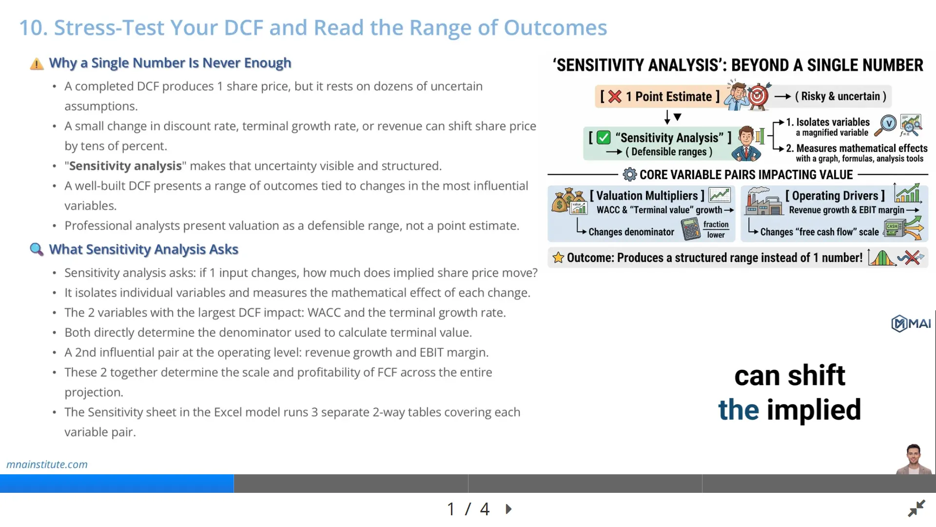
The first discipline in DCF sensitivity analysis is admitting that the base case is only one version of the future.

A DCF model may produce one share price, but that number rests on revenue growth, margin progression, reinvestment needs, terminal value assumptions, and the discount rate.

Each assumption may be reasonable on its own, but the combined result can still be fragile.

If the value changes dramatically after a small move in one input, the analyst must understand why before presenting the model.

For example, assume a company has a base case implied share price of 100 dollars.

If a one percentage point increase in WACC lowers the implied value to 78 dollars, the valuation is highly exposed to discount rate assumptions.

If a modest reduction in terminal growth rate lowers the value to 85 dollars, the terminal value assumption is also carrying a large share of the conclusion.

Neither result means the model is wrong.

It means the analyst should not present 100 dollars as a false certainty.

A better conclusion is that the company is worth 78 to 120 dollars depending on discount rate, growth, and operating performance assumptions.

That range is more honest and more useful than a single number because DCF sensitivity analysis tells the reader what drives the result.

This is why sensitivity analysis financial modeling is not a formatting exercise.

It is an analytical process that helps the analyst translate uncertainty into a valuation range.

What Sensitivity Analysis Asks

DCF sensitivity analysis asks a narrow but powerful question.

If one input changes, how much does the implied share price move?

The point of DCF sensitivity analysis is not to rewrite the entire investment thesis every time one cell changes.

The point is to isolate the mathematical impact of a single variable or a pair of variables.

In a DCF model, the most common variables to test are WACC, terminal growth rate, exit multiple, revenue growth, and EBIT margin.

WACC and terminal growth rate are usually tested together because both affect the denominator in the Gordon Growth terminal value formula.

A small difference between WACC and terminal growth can create a large terminal value.

A wider difference can reduce terminal value sharply.

Revenue growth and EBIT margin are tested together because they drive the scale and profitability of free cash flow during the explicit forecast period.

Higher revenue growth without margin support may not produce as much free cash flow as the headline growth rate suggests.

Higher margin without credible revenue expansion may also be difficult to defend.

The most useful DCF sensitivity analysis table therefore does not just show random combinations.

It tests the assumptions that actually control the valuation conclusion.

The Three Scenario Tables a DCF Model Should Contain

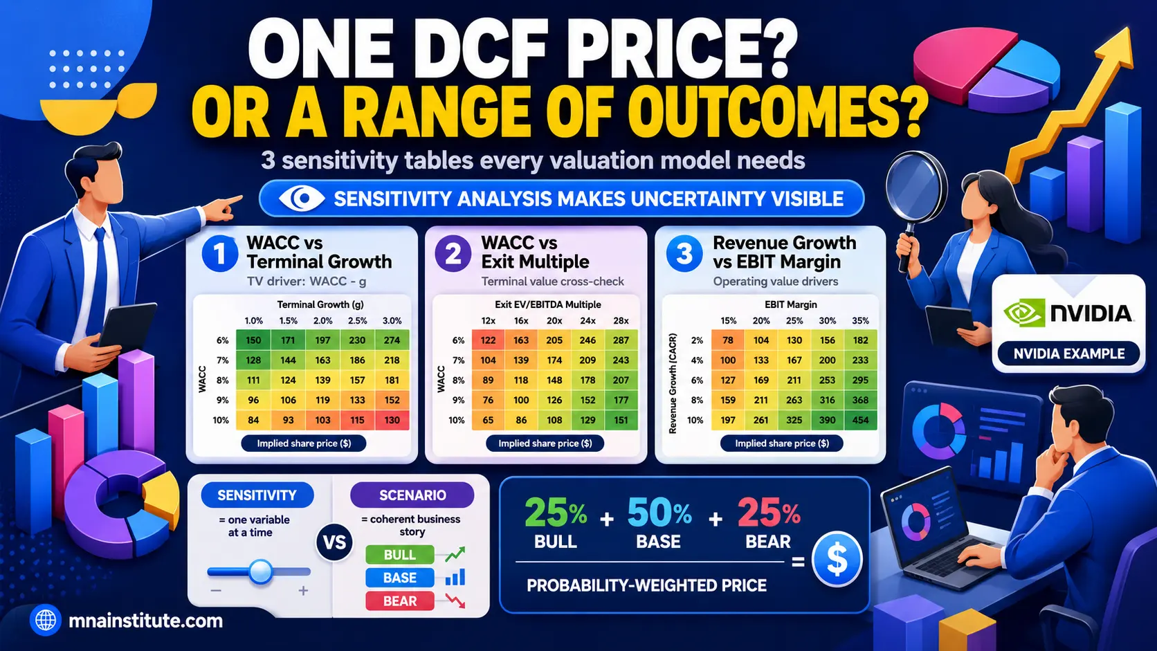
The course model uses three practical DCF sensitivity analysis tables because each table tests a different part of the valuation logic.

The first table tests WACC against terminal growth rate.

The second table tests WACC against the exit EV to EBITDA multiple.

The third table tests operating performance by crossing revenue growth against EBIT margin.

Together, the three tables separate discount rate risk, terminal value methodology risk, and operating forecast risk.

That separation matters because DCF sensitivity analysis shows that not all valuation uncertainty comes from the same source.

A company may have strong operating visibility but high discount rate sensitivity because terminal value dominates total value.

Another company may have stable WACC assumptions but wide revenue and margin uncertainty because the business is early in its growth cycle.

A good DCF sensitivity analysis makes these distinctions visible.

It prevents the analyst from explaining every valuation movement with the same generic comment.

Table 1: WACC and terminal growth rate

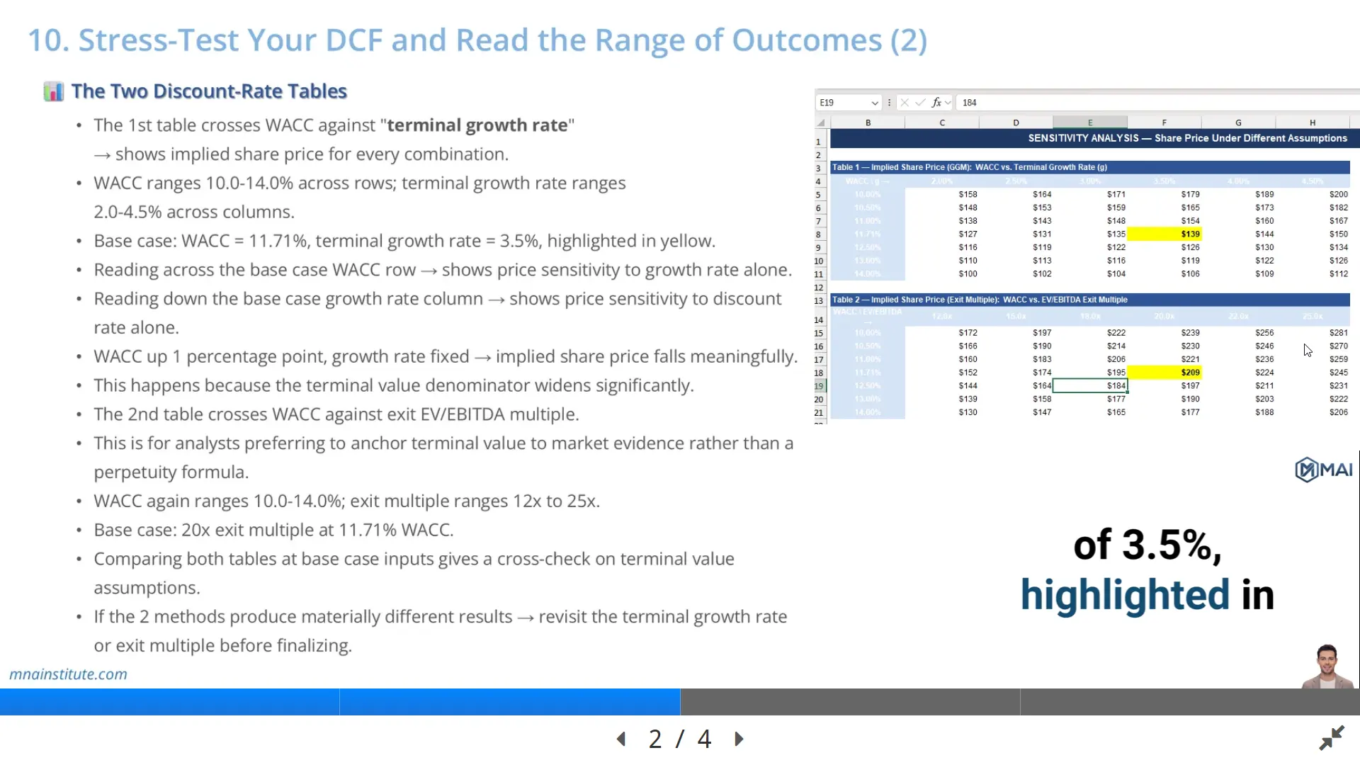
The first DCF sensitivity analysis table crosses WACC against terminal growth rate.

In the course model, WACC ranges from 10.0 percent to 14.0 percent, while the terminal growth rate ranges from 2.0 percent to 4.5 percent.

The base case sits at WACC of 11.71 percent and terminal growth rate of 3.5 percent.

Reading across the row shows how the valuation changes when the terminal growth rate changes while WACC stays constant.

Reading down the column shows how the valuation changes when WACC changes while terminal growth rate stays constant.

This is the core of WACC sensitivity analysis because the discount rate determines how aggressively future cash flows are brought back to present value.

The terminal growth rate determines how large the continuing value becomes after the explicit forecast period.

When both move at the same time, the impact can be much larger than a junior analyst expects.

Table 2: WACC and exit EV to EBITDA multiple

The second DCF sensitivity analysis table is designed for analysts who want to cross-check the terminal value using a market-based exit multiple.

Instead of relying only on the perpetuity growth method, the table applies an exit EV to EBITDA multiple to final-year EBITDA.

In the course model, WACC again ranges from 10.0 percent to 14.0 percent, while the exit multiple ranges from 12x to 25x.

The base case uses a 20x exit multiple at 11.71 percent WACC.

This table is especially useful when valuing businesses where public market multiples or precedent transaction multiples provide relevant market evidence.

It also gives the analyst a practical cross-check against the perpetuity growth model.

If the WACC and terminal growth table produces a very different value from the WACC and exit multiple table, the analyst should revisit the terminal assumptions before finalizing the conclusion.

The purpose is not to force both methods to produce the same value.

The purpose is to understand why they differ and whether the difference is justified.

Table 3: revenue growth and EBIT margin

The third DCF sensitivity analysis table moves from discounting assumptions to operating assumptions.

It tests how implied share price changes when revenue growth and EBIT margin move together.

This matters because free cash flow is not driven by growth alone.

It is driven by growth, margin, tax, reinvestment, and working capital needs.

For a high-growth semiconductor company, revenue growth may depend on data center demand, AI infrastructure spending, customer concentration, and supply availability.

EBIT margin may depend on pricing power, product mix, manufacturing costs, and competitive pressure.

A revenue growth and EBIT margin table forces the analyst to ask whether the operating forecast is internally consistent.

A model that assumes strong revenue growth but collapsing margins tells a different story from one that assumes moderate growth with expanding profitability.

That difference should be explained before the valuation is presented.

The Two Discount-Rate Tables

The two discount-rate tables are the part of DCF sensitivity analysis that often receives the most attention.

That is because the present value of cash flows and terminal value is highly sensitive to the discount rate.

A higher WACC reduces the present value of future cash flows.

A lower WACC increases it.

This effect is especially strong when much of the value is generated far in the future.

High-growth companies often have that profile because large portions of their value come from cash flows expected after the early projection years.

That makes the discount rate table more than a mechanical Excel output.

It becomes a test of whether the investment case can survive a higher required return.

The WACC and terminal growth rate table answers one question.

How much of the valuation depends on the spread between WACC and long-run growth?

The WACC and exit multiple table answers a second question.

How much of the valuation depends on the market multiple assumed at the end of the forecast period?

A strong analyst reads both DCF sensitivity analysis tables together.

If the base case value only works at a low WACC and a high terminal growth rate, the conclusion may be too aggressive.

If the exit multiple table supports a similar range using market evidence, the conclusion becomes easier to defend.

If the two tables conflict, the analyst must explain whether the market multiple, the terminal growth rate, or the explicit forecast is doing too much work.

Scenario Analysis Builds a Narrative

DCF sensitivity analysis changes one variable or a pair of variables.

Scenario analysis changes several assumptions at the same time and connects them to a coherent business story.

This distinction is essential.

A sensitivity table can show what happens if WACC rises to 13 percent.

It does not explain why WACC would rise to 13 percent, what would happen to demand, or whether margin pressure would appear at the same time.

DCF scenario analysis provides that missing narrative layer.

In a Bull case, the analyst might assume stronger revenue growth, stable pricing power, expanding EBIT margin, and a lower or unchanged WACC.

Those assumptions can be consistent if the business story is that demand is stronger than expected and competitive pressure remains contained.

In a Bear case, the analyst might assume slower revenue growth, compressed EBIT margin, lower terminal growth, and a higher WACC.

Those assumptions can be consistent if the story is that demand slows, competitors intensify pricing pressure, and earnings visibility deteriorates.

The mistake is combining assumptions that do not belong together.

A Bear revenue case with a Bull margin case may be possible, but it needs a specific explanation.

For example, it might make sense if the company deliberately exits low-margin revenue and focuses only on profitable segments.

Without that explanation, the scenario looks like a spreadsheet compromise rather than an investment view.

Professional DCF scenario analysis therefore demands two tests.

First, each scenario must be numerically coherent.

Second, each scenario must be commercially believable.

Probability-Weighted Price

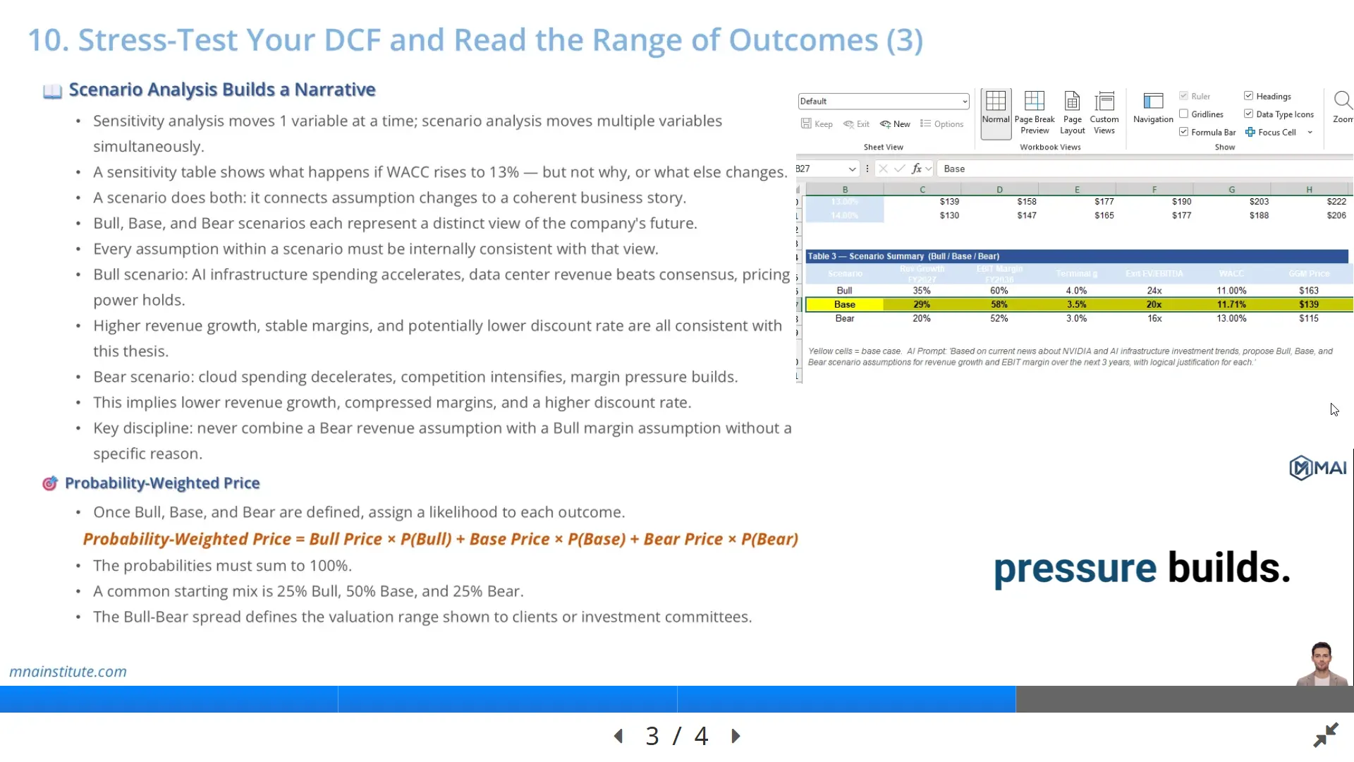
Once Bull, Base, and Bear scenarios are defined, the analyst can calculate a probability-weighted implied share price.

The formula is simple.

Probability-weighted price equals Bull price multiplied by the Bull probability, plus Base price multiplied by the Base probability, plus Bear price multiplied by the Bear probability.

The probabilities must sum to 100 percent.

A common starting point is 25 percent Bull, 50 percent Base, and 25 percent Bear.

That distribution does not need to be used in every model.

The correct distribution depends on the analyst’s view of the risk profile.

If downside risk is unusually high, the Bear probability may need to be greater than 25 percent.

If the company has strong contracted revenue, stable margin, and low execution risk, the Base probability may deserve more weight.

The probability-weighted value is not a replacement for the scenario range.

It is a summary statistic that sits inside the range.

The range tells the reader what could happen.

The probability-weighted price tells the reader where the analyst’s expected value sits after considering the likelihood of each outcome.

This approach is especially useful when presenting to an investment committee because it separates upside potential from expected value.

A stock can have an exciting Bull case and still be unattractive if the probability-weighted value is below the current market price.

A stock can also look expensive in the base case but still be interesting if downside is limited and upside is both large and plausible.

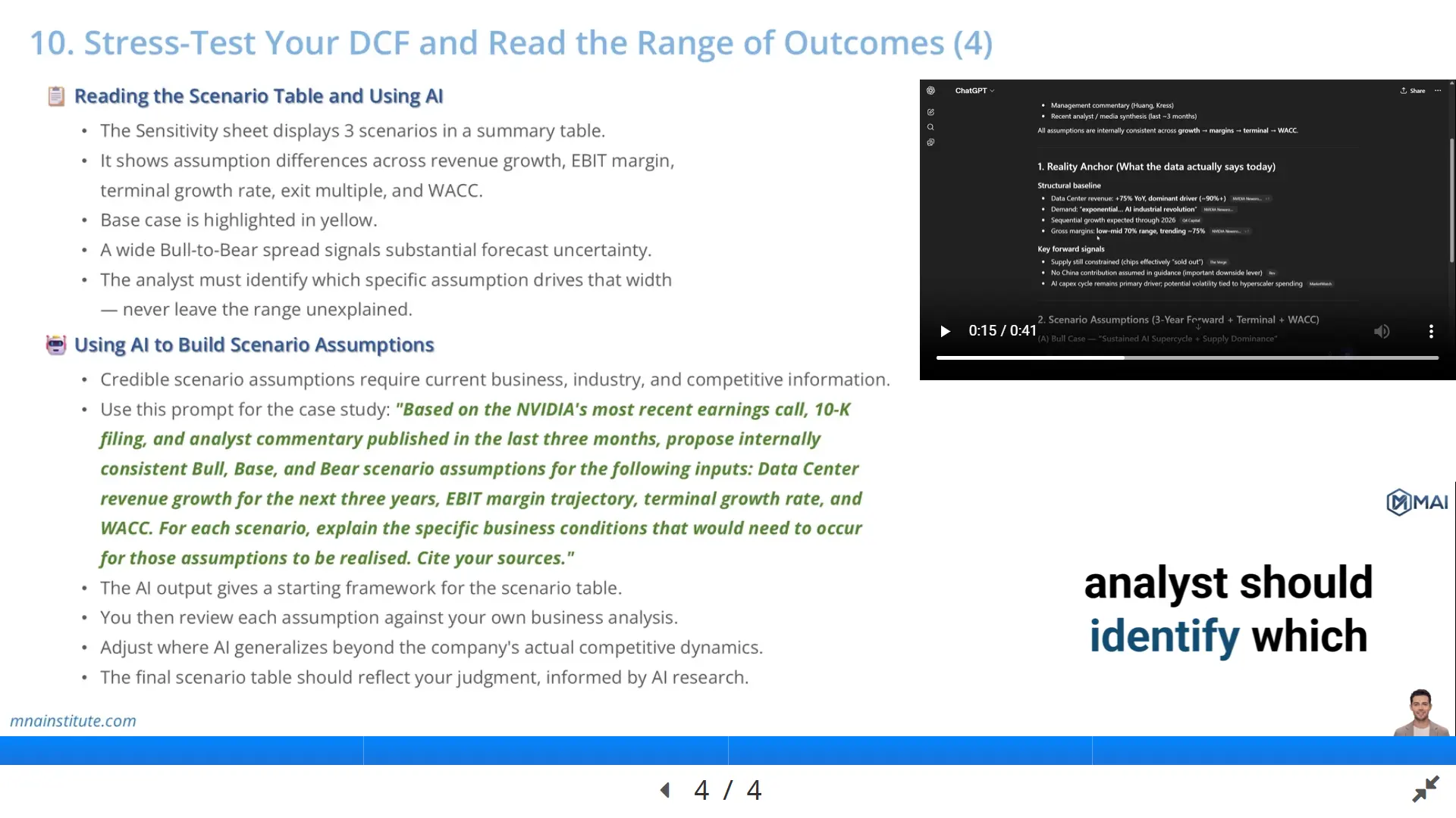
Reading the Scenario Table and Using AI

The scenario table should not be read as a decorative summary page.

It should be read as the final audit of the valuation thesis.

The table should show the key assumptions for Bull, Base, and Bear cases side by side.

At minimum, it should include revenue growth, EBIT margin, terminal growth rate, exit multiple, WACC, and implied share price.

A clear table allows the reader to see which assumptions move together and which assumptions explain the valuation spread.

A wide spread between Bull and Bear prices is not a problem by itself.

It becomes a problem only when the analyst cannot identify the assumption that creates the width.

For example, if most of the spread comes from terminal growth rate, the discussion should focus on terminal value credibility.

If most of the spread comes from EBIT margin, the discussion should focus on operating leverage, pricing power, and cost structure.

If most of the spread comes from WACC, the discussion should focus on risk, rates, capital structure, and market volatility.

AI can help build an initial scenario framework for DCF sensitivity analysis because it can summarize earnings calls, filings, news, and analyst commentary faster than manual review.

However, AI should not be allowed to produce the final assumptions without verification.

The analyst should use AI output as a research starting point, not as a substitute for judgment.

A credible AI-assisted workflow has three steps.

First, ask AI to identify business conditions that would support Bull, Base, and Bear cases.

Second, ask AI to tie those conditions to measurable inputs such as revenue growth, EBIT margin, WACC, and terminal growth rate.

Third, compare every proposed assumption against filings, management guidance, consensus data, and the analyst’s own model logic.

This is how AI can support sensitivity analysis financial modeling without weakening analytical discipline.

Using AI to Build Scenario Assumptions

The best prompt for DCF scenario analysis should not simply ask AI to make a Bull, Base, and Bear case.

That usually produces generic assumptions.

A better prompt specifies the company, the time period, the sources to review, and the exact inputs that must be estimated.

For a high-growth semiconductor case, the prompt might ask for data center revenue growth, EBIT margin trajectory, terminal growth rate, and WACC assumptions for each scenario.

It should also ask AI to explain the business conditions required for each assumption to be realized.

That last instruction is the most important part of AI-supported DCF sensitivity analysis.

A Bull case is not a column of high numbers.

It is a set of assumptions that become possible only if specific business conditions occur.

A Bear case is not a column of pessimistic numbers.

It is a set of assumptions that become possible if demand, pricing, margin, or risk conditions deteriorate.

After receiving AI output, the analyst should revise the scenario assumptions manually.

AI may generalize from market commentary and miss company-specific constraints.

It may overstate consensus if it does not distinguish between outdated commentary and current guidance.

It may also treat all risks as equally important, even when one risk dominates the model.

The final DCF sensitivity analysis must therefore reflect the analyst’s own judgment.

AI can widen the research funnel, but the analyst owns the valuation conclusion.

A Practical Interpretation Checklist

• Check whether the base case sits near the center of the DCF sensitivity table or at an aggressive edge.
• Check whether WACC sensitivity analysis shows a stable range or a valuation that collapses under a small rate increase.
• Compare the Gordon Growth terminal value output with the exit multiple method output.
• Ask whether revenue growth and EBIT margin assumptions are commercially consistent.
• Identify the one assumption that explains the largest portion of the Bull to Bear spread.
• Use probability-weighted valuation as a summary, but never hide the full scenario range.
• Document every assumption that defines the valuation boundary.
• Use AI for research and scenario framing, but verify all assumptions against source data.

Related Courses

This topic sits inside practical valuation work because a completed DCF model must be tested before it can support an investment conclusion.

The related courses below connect the modeling, statement analysis, and transaction context behind the sensitivity work.

• Financial Modeling and Valuation Course with AI and Excel
• Financial Statement Analysis Course with AI for Equity Research
• 3-Statement Financial Modeling Course with AI
• Mergers and Acquisitions Online Course
• M&A Due Diligence Course
• Post Merger Integration Course

Sources

• CFA Institute, Equity Valuation: Applications and Processes
• CFA Institute, Financial Analysis Techniques
• Aswath Damodaran, Probabilistic Approaches in Valuation: Scenario Analysis, Decision Trees and Simulations
• McKinsey & Company, The right role for multiples in valuation